from os import listdirfrom os.path import isfile, joinimport pandas as pdimport numpy as npimport matplotlib.pyplot as pltimport polars as plimport globfrom scipy.stats import pearsonr, spearmanrimport seaborn as snsfrom math import piimport osimport requestspd.set_option('display.max_columns', None)plt.style.use('dark_background')!pip install awpy
Requirement already satisfied: awpy in /usr/local/lib/python3.11/dist-packages (2.0.2)
Requirement already satisfied: click>=8.1.8 in /usr/local/lib/python3.11/dist-packages (from awpy) (8.2.1)
Requirement already satisfied: demoparser2>=0.38.0 in /usr/local/lib/python3.11/dist-packages (from awpy) (0.39.0)
Requirement already satisfied: loguru>=0.7.3 in /usr/local/lib/python3.11/dist-packages (from awpy) (0.7.3)
Requirement already satisfied: matplotlib>=3.10.0 in /usr/local/lib/python3.11/dist-packages (from awpy) (3.10.0)
Requirement already satisfied: networkx>=3.4.2 in /usr/local/lib/python3.11/dist-packages (from awpy) (3.5)
Requirement already satisfied: numpy>=2.0.0 in /usr/local/lib/python3.11/dist-packages (from awpy) (2.0.2)
Requirement already satisfied: pillow>=11.1.0 in /usr/local/lib/python3.11/dist-packages (from awpy) (11.2.1)
Requirement already satisfied: polars>=1.22.0 in /usr/local/lib/python3.11/dist-packages (from awpy) (1.30.0)
Requirement already satisfied: requests>=2.32.3 in /usr/local/lib/python3.11/dist-packages (from awpy) (2.32.3)
Requirement already satisfied: scipy>=1.15.0 in /usr/local/lib/python3.11/dist-packages (from awpy) (1.15.3)
Requirement already satisfied: tqdm>=4.67.1 in /usr/local/lib/python3.11/dist-packages (from awpy) (4.67.1)
Requirement already satisfied: pandas>=1.5.0 in /usr/local/lib/python3.11/dist-packages (from demoparser2>=0.38.0->awpy) (2.2.2)
Requirement already satisfied: pyarrow in /usr/local/lib/python3.11/dist-packages (from demoparser2>=0.38.0->awpy) (18.1.0)
Requirement already satisfied: contourpy>=1.0.1 in /usr/local/lib/python3.11/dist-packages (from matplotlib>=3.10.0->awpy) (1.3.2)
Requirement already satisfied: cycler>=0.10 in /usr/local/lib/python3.11/dist-packages (from matplotlib>=3.10.0->awpy) (0.12.1)
Requirement already satisfied: fonttools>=4.22.0 in /usr/local/lib/python3.11/dist-packages (from matplotlib>=3.10.0->awpy) (4.58.1)
Requirement already satisfied: kiwisolver>=1.3.1 in /usr/local/lib/python3.11/dist-packages (from matplotlib>=3.10.0->awpy) (1.4.8)
Requirement already satisfied: packaging>=20.0 in /usr/local/lib/python3.11/dist-packages (from matplotlib>=3.10.0->awpy) (24.2)
Requirement already satisfied: pyparsing>=2.3.1 in /usr/local/lib/python3.11/dist-packages (from matplotlib>=3.10.0->awpy) (3.2.3)
Requirement already satisfied: python-dateutil>=2.7 in /usr/local/lib/python3.11/dist-packages (from matplotlib>=3.10.0->awpy) (2.9.0.post0)
Requirement already satisfied: charset-normalizer<4,>=2 in /usr/local/lib/python3.11/dist-packages (from requests>=2.32.3->awpy) (3.4.2)
Requirement already satisfied: idna<4,>=2.5 in /usr/local/lib/python3.11/dist-packages (from requests>=2.32.3->awpy) (3.10)
Requirement already satisfied: urllib3<3,>=1.21.1 in /usr/local/lib/python3.11/dist-packages (from requests>=2.32.3->awpy) (2.4.0)
Requirement already satisfied: certifi>=2017.4.17 in /usr/local/lib/python3.11/dist-packages (from requests>=2.32.3->awpy) (2025.4.26)
Requirement already satisfied: pytz>=2020.1 in /usr/local/lib/python3.11/dist-packages (from pandas>=1.5.0->demoparser2>=0.38.0->awpy) (2025.2)
Requirement already satisfied: tzdata>=2022.7 in /usr/local/lib/python3.11/dist-packages (from pandas>=1.5.0->demoparser2>=0.38.0->awpy) (2025.2)
Requirement already satisfied: six>=1.5 in /usr/local/lib/python3.11/dist-packages (from python-dateutil>=2.7->matplotlib>=3.10.0->awpy) (1.17.0)
Demo parsing Snippets for local use.
Due to the size and availability of .dem files. Providing code that performs our analysis from the point of getting the .dems is expensive. As a result below is some generalized code that can be used to parse demos for our purposes, given you garner the .dem files from the sources we provide.
import osfrom awpy import Demoimport polars as pl#set up folders for your usedemos_folder ="folder_of_demos"output_folder ="output_folder_for_parsed_demos"os.makedirs(output_folder, exist_ok=True)#dataframes we gathered for our analyis. Change this to contain as many or as few data frames as you'd like.dataframes_to_save = ["rounds", "grenades", "kills", "damages", "bomb", "smokes", "infernos", "shots"]def parse_demos(in_folder, out_folder, verbose=True): files = [f for f in os.listdir(in_folder) if f.endswith(".dem")] #look for demo files in folderfor f in files: path = os.path.join(in_folder, f)if verbose:print(f"Parsing {f}")try: demo = Demo(path, verbose=verbose) #create a demo object from demo file demo.parse() #parse demo to get dataframes as attributes name = os.path.splitext(f)[0]for df_name in dataframes_to_save: df =getattr(demo, df_name, None) #for each dataframe name, get that from the parsed demo and save it as a csvifisinstance(df, pl.DataFrame) and df.height >0: out_path = os.path.join(out_folder, f"{name}_{df_name}.csv") df.write_csv(out_path)if verbose:print(f"Saved: {out_path}")exceptExceptionas e:print(f"Problem with {f}: {e}")#you'll notice some attributes (sounds often) are broken#demos are often corrupted for one reason or another#if a dataframe is empty, you unfortunately can't use itdef filter_by_tick(folder, keyword, every_n, verbose=True):for f in os.listdir(folder):if keyword in f and f.endswith(".csv"): path = os.path.join(folder, f)if verbose:print(f"Filtering {f}") df = pl.read_csv(path)if"tick"in df.columns: df = df.filter(pl.col("tick") % every_n ==0) df.write_csv(path)if verbose:print(f"Saved filtered: {f}")else:if verbose:print(f"No 'tick' column in {f}, skipped")#Example usage:#parse_demos(demos_folder, output_folder, verbose=True)#filter_by_tick(output_folder, "grenades", 8, verbose=True)
The github we link to below has done this for every match at IEM Dallas 2025 that was played by either Vitality or Mouz Rank 1 and Rank 2, Winner and Runner Up respectively.
# for a given repo containing CSVs, this function downloads all to our google collab space.def download_csvs(user, repo, output_folder): os.makedirs(output_folder, exist_ok=True) tree_url =f"https://api.github.com/repos/{user}/{repo}/git/trees/main?recursive=1" raw_base =f"https://raw.githubusercontent.com/{user}/{repo}/main/" r = requests.get(tree_url) csv_files = [f["path"] for f in r.json()["tree"] if f["path"].endswith(".csv")]forfilein csv_files: url = raw_base +file dest = os.path.join(output_folder, os.path.basename(file)) file_data = requests.get(url)if file_data.ok:withopen(dest, "wb") as f: f.write(file_data.content)print(f"Downloaded: {file}")else:print(f"Failed: {file}")
def get_df(team_name, file_type, file_path ="/content/DLfromGitHubTesting/", roster = []): proper_file_types = ["bomb", "damages", "grenades", "infernos", "kills", "rounds", "shots", "smokes"]if file_type notin proper_file_types:returnf"Invalid file type please use from {proper_file_types}"#just get match files which include "vs" files = [f for f in listdir(file_path) if isfile(join(file_path, f)) and"vs"in f]#filter down to files that have team_files = [f for f in files if team_name in f and file_type in f] list_df = []for filename in team_files: full_path = file_path + filename team1, rest = filename.split("-vs-",1) team2 = rest.split("-")[0] team1 = team1.strip().lower() team2 = team2.strip().lower()if team2 =="the": team2 ="mongolz"#get map name map_parts = rest.split("-")for part in map_parts:if part in ['m1', 'm2', 'm3']: # match indicators map_played = map_parts[map_parts.index(part) +1].split("_")[0]break df = pd.read_csv(full_path) df["map"] = map_played df["opponent"] = team2 if team1 == team_name else team1 list_df.append(df)#combine list of df into one large df combined_df = pd.concat(list_df, axis =0)#filter for players in rosteriflen(roster) >=1:if file_type =="kills"or file_type =="damages": combined_df = combined_df[combined_df["attacker_name"].isin(roster)]elif file_type =="grenades": combined_df = combined_df[combined_df["thrower"].isin(roster)]elif file_type =="infernos": combined_df = combined_df[combined_df["thrower_name"].isin(roster)]#drop steamid steam_id_col = [col for col in combined_df.columns if"steamid"in col] combined_df = combined_df.drop(columns = steam_id_col, axis =1)return combined_df
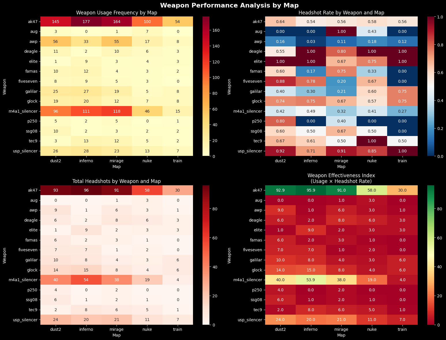
Create weapon usage rate and its performace across maps played. This helps us see how each weapons were used and if each weapon performed better or worse depending on the map.
               win_rate  total_rounds  wins
team     side
MOUZ     ct       74.01           118    79
         t        54.82           107    56
Vitality ct       53.29           141    81
         t        54.25           129    74
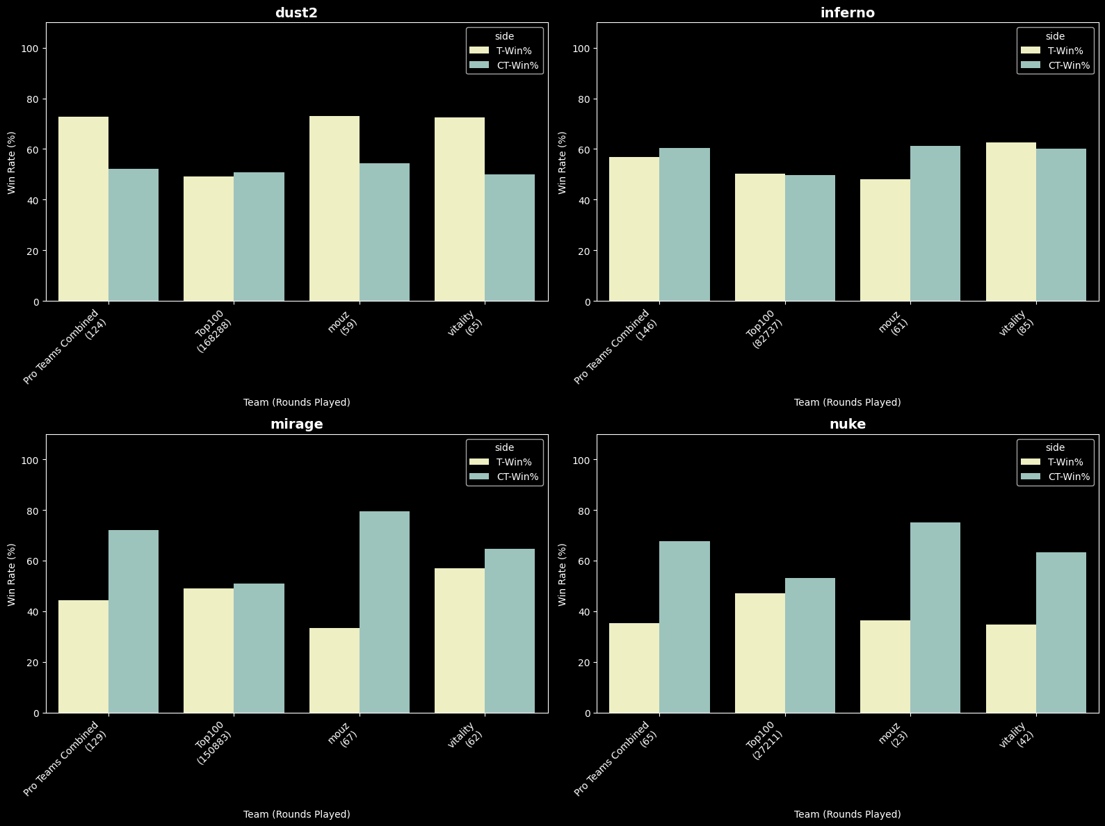
Convert pro rounds dataset into a format that is similar to the Top 100 dataset. It calculates win percentages per side per map. The column names were matched to the 2nd dataset which allows for easy concatenation
Although the table above is easier to see on the eye, we had to melt the dataset for visualization. We melted on map, team, and rounds played and set values as side and win rate.
def melt_df(df, id_vars, value_vars, var_name, value_name): melted_df = df.melt(id_vars=id_vars, value_vars=value_vars, var_name=var_name, value_name=value_name) melted_df = melted_df.sort_values(by=id_vars)return melted_df#just get columns to combinesimple_pro_map_stats = pro_map_statistics[["map", "Team", "T-Win%", "CT-Win%", "Rounds-Played"]]#just get maps played in IEM Dallasmaps_statistics = maps_statistics[maps_statistics["map"].isin(simple_pro_map_stats["map"].unique())]combined = pd.concat([maps_statistics, simple_pro_map_stats], ignore_index=True)combined = combined.drop(["Play Rate"], axis=1)melted = melt_df(combined, ["map", "Team","Rounds-Played"], ["T-Win%", "CT-Win%"], "side", "win_rate")melted.head()
map
Team
Rounds-Played
side
win_rate
14
dust2
Pro Teams Combined
124
T-Win%
72.73
33
dust2
Pro Teams Combined
124
CT-Win%
52.17
0
dust2
Top100
168288
T-Win%
49.20
19
dust2
Top100
168288
CT-Win%
50.80
4
dust2
mouz
59
T-Win%
73.10
maps = melted["map"].unique()maps = [map_name for map_name in maps if map_name.lower() !='train'] # We dont have top 100 data for train# Create 2x2 subplot layoutfig, axes = plt.subplots(2, 2, figsize=(16, 12))axes = axes.flatten()for i, map_name inenumerate(maps[:4]): map_data = melted[melted["map"] == map_name] ax = axes[i] sns.barplot(map_data, x="Team", y="win_rate", hue="side", ax=ax, palette={"T-Win%": "#f5f6bc", "CT-Win%": "#96cac1"} ) ax.set_title(map_name, fontsize=14, fontweight='bold') ax.set_ylim(0, 110) ax.set_ylabel("Win Rate (%)")# Get rounds played for each team team_rounds = map_data.groupby(["Team"])["Rounds-Played"].first() ax.set_xlabel("Team (Rounds Played)")# Set x-axis labels with rounds played teams_in_plot_order = map_data["Team"].unique() labels = [f"{team}\n({team_rounds[team]})"for team in teams_in_plot_order] ax.set_xticklabels(labels, rotation=45, ha='right')# Hide any unused subplots if there are fewer than 4 mapsfor j inrange(len(maps), 4): axes[j].set_visible(False)plt.tight_layout()plt.show()
UserWarning: set_ticklabels() should only be used with a fixed number of ticks, i.e. after set_ticks() or using a FixedLocator.
  ax.set_xticklabels(labels, rotation=45, ha='right')
<ipython-input-22-3435786538>:32: UserWarning: set_ticklabels() should only be used with a fixed number of ticks, i.e. after set_ticks() or using a FixedLocator.
  ax.set_xticklabels(labels, rotation=45, ha='right')
<ipython-input-22-3435786538>:32: UserWarning: set_ticklabels() should only be used with a fixed number of ticks, i.e. after set_ticks() or using a FixedLocator.
  ax.set_xticklabels(labels, rotation=45, ha='right')
<ipython-input-22-3435786538>:32: UserWarning: set_ticklabels() should only be used with a fixed number of ticks, i.e. after set_ticks() or using a FixedLocator.
  ax.set_xticklabels(labels, rotation=45, ha='right')
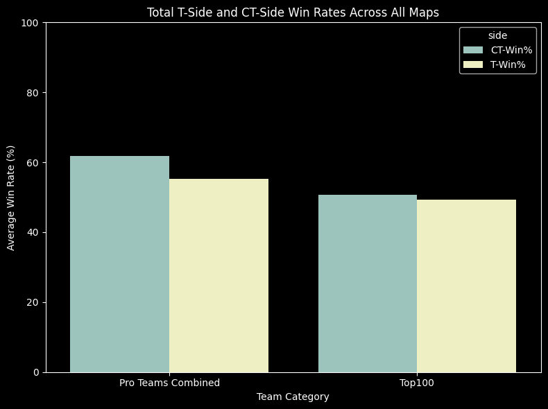
top_and_pro_stats = melted[melted["Team"].isin(["Top100", "Pro Teams Combined"])]aggregated_stats = top_and_pro_stats.groupby(["Team", "side"]).apply(lambda x: (x["win_rate"] * x["Rounds-Played"]).sum() / x["Rounds-Played"].sum()).reset_index(name="win_rate")aggregated_statsplt.figure(figsize=(8, 6))sns.barplot(data=aggregated_stats, x="Team", y="win_rate", hue="side", palette={"T-Win%": "#f5f6bc", "CT-Win%": "#96cac1"})plt.title("Total T-Side and CT-Side Win Rates Across All Maps")plt.xlabel("Team Category")plt.ylabel("Average Win Rate (%)")plt.ylim(0, 100) # Win rates are percentages, so limit to 0-100plt.tight_layout()plt.show()
DeprecationWarning: DataFrameGroupBy.apply operated on the grouping columns. This behavior is deprecated, and in a future version of pandas the grouping columns will be excluded from the operation. Either pass `include_groups=False` to exclude the groupings or explicitly select the grouping columns after groupby to silence this warning.
  aggregated_stats = top_and_pro_stats.groupby(["Team", "side"]).apply(lambda x: (x["win_rate"] * x["Rounds-Played"]).sum() / x["Rounds-Played"].sum()).reset_index(name="win_rate")
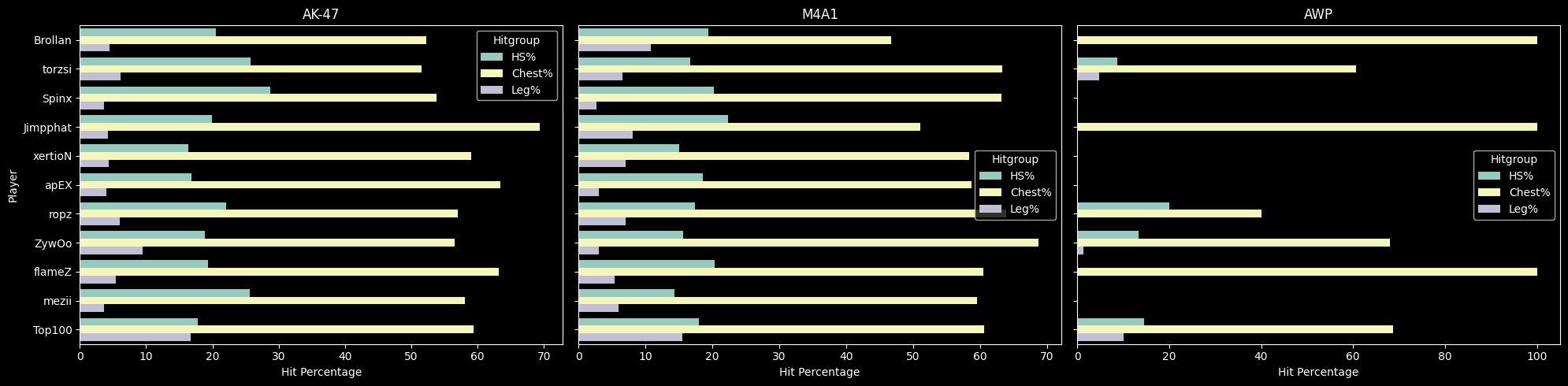
Similar to the maps function, we had to format the damages dataset into a format similar to the Top 100 weapons dataset. Grouped by attacker_name, weapon, and hitgoup allowed us to calculate where a player shot for each weapon.
We decided to aggregate some body parts based on damage multipliers.
df_kills_vitality
assistedflash
assister_X
assister_Y
assister_Z
assister_health
assister_place
assister_name
assister_side
attacker_X
attacker_Y
attacker_Z
attacker_health
attacker_place
attacker_name
attacker_side
attackerblind
attackerinair
ct_side
distance
dmg_armor
dmg_health
dominated
headshot
hitgroup
noreplay
noscope
penetrated
revenge
t_side
thrusmoke
tick
victim_X
victim_Y
victim_Z
victim_health
victim_place
victim_name
victim_side
weapon
weapon_fauxitemid
weapon_itemid
weapon_originalowner_xuid
wipe
round_num
map
opponent
1
False
NaN
NaN
NaN
NaN
NaN
NaN
NaN
716.55760
2248.59640
136.03139
62.0
Banana
apEX
t
False
False
ct
14.876597
0
99
0
True
head
False
False
0
0
t
False
7062
789.90740
2834.02340
143.47398
89
BombsiteB
Spinx
ct
glock
17293822569165815812
2.227010e+10
NaN
0
1
inferno
mouz
2
False
NaN
NaN
NaN
NaN
NaN
NaN
NaN
794.72510
2626.90480
136.03148
66.0
BombsiteB
mezii
t
False
False
ct
20.576242
0
92
0
True
head
False
False
0
0
t
False
7078
66.07632
2977.64280
161.03125
31
BombsiteB
Brollan
ct
glock
17293822569125838852
4.045856e+10
NaN
0
1
inferno
mouz
8
False
NaN
NaN
NaN
NaN
NaN
NaN
NaN
1446.48160
474.70830
120.00048
100.0
TopofMid
mezii
t
False
False
ct
9.128391
28
50
0
True
head
False
False
0
0
t
False
12652
1281.24700
793.75006
141.53140
3
TopofMid
Spinx
ct
glock
17293822569125838852
4.045856e+10
NaN
0
2
inferno
mouz
13
False
NaN
NaN
NaN
NaN
NaN
NaN
NaN
430.28317
1773.78740
226.03125
100.0
Banana
ZywOo
t
False
False
ct
13.389605
15
109
0
True
head
False
False
0
0
t
False
16711
759.57294
2170.76050
136.03130
94
Banana
xertioN
ct
ak47
17293822569179447303
3.722510e+10
NaN
0
3
inferno
mouz
15
False
410.16513
1790.5015
226.03125
0.0
Banana
ZywOo
t
615.51605
1962.37840
136.03125
100.0
Banana
mezii
t
False
False
ct
11.596359
3
27
0
False
left_arm
False
False
0
0
t
False
16850
828.45860
2366.28830
140.08430
19
BombsiteB
Spinx
ct
ak47
17293822569144582151
4.376131e+10
NaN
0
3
inferno
mouz
...
...
...
...
...
...
...
...
...
...
...
...
...
...
...
...
...
...
...
...
...
...
...
...
...
...
...
...
...
...
...
...
...
...
...
...
...
...
...
...
...
...
...
...
...
...
...
155
False
NaN
NaN
NaN
NaN
NaN
NaN
NaN
85.99862
-2094.97000
-39.96875
100.0
PalaceInterior
ropz
t
False
False
ct
29.220425
0
137
0
True
head
False
False
0
0
t
False
208567
-982.36290
-2503.90500
-167.96875
43
CTSpawn
910-
ct
ak47
17293822569144582151
4.034253e+10
NaN
0
24
mirage
mongolz
156
False
NaN
NaN
NaN
NaN
NaN
NaN
NaN
61.99465
-2203.64820
-39.96875
78.0
PalaceInterior
ropz
t
False
False
ct
32.096325
15
106
0
True
head
False
False
0
0
t
False
208641
-882.37335
-1374.07890
-167.96875
99
Jungle
bLitz
ct
ak47
17293822569144582151
4.034253e+10
NaN
0
24
mirage
mongolz
158
False
NaN
NaN
NaN
NaN
NaN
NaN
NaN
-687.98413
-911.75146
-228.08936
99.0
Connector
apEX
t
False
False
ct
33.491673
0
136
0
True
head
False
False
0
0
t
True
209827
-788.93567
-2226.06760
-179.96875
100
BombsiteA
Mzinho
ct
ak47
17293822569144582151
4.034253e+10
NaN
0
24
mirage
mongolz
159
False
NaN
NaN
NaN
NaN
NaN
NaN
NaN
-419.02527
-1676.79870
-167.96875
67.0
BombsiteA
flameZ
t
False
False
ct
18.067097
15
108
0
True
head
False
False
0
0
t
False
212756
-1098.81750
-1467.72010
-164.33008
40
CTSpawn
Senzu
ct
ak47
17293822569179447303
3.722510e+10
NaN
0
24
mirage
mongolz
161
False
NaN
NaN
NaN
NaN
NaN
NaN
NaN
-1061.95540
-2464.47390
-167.96875
99.0
CTSpawn
apEX
t
False
False
ct
22.062593
15
107
0
True
head
False
False
0
0
t
False
214832
-240.61316
-2179.67380
-170.06927
48
BombsiteA
Techno4K
ct
ak47
17293822569144582151
4.034253e+10
NaN
0
24
mirage
mongolz
985 rows × 46 columns
#get weapons_statistics df for proplayersdef get_weapon_hit_where(df, team_name, weapons): copy = df.copy() num_rounds = df_rounds_mouz.shape[0] if team_name.lower() =="mouz"else df_rounds_vitality.shape[0] copy = copy[copy["weapon"].isin(weapons)] hit_count = copy.groupby(["attacker_name","weapon", "hitgroup"]).size().reset_index(name ="hit_count") total_hits = hit_count.groupby(["attacker_name", "weapon"])["hit_count"].sum().reset_index(name="total_hits") merged = hit_count.merge(total_hits, on = ["attacker_name", "weapon"]) merged["hit_percentage"] =round(merged["hit_count"] / merged["total_hits"] *100,1) pivot = merged.pivot(index = ["attacker_name", "weapon"], columns = ["hitgroup"], values ="hit_percentage").fillna(0).reset_index()#combine legs to one leg col and combine arms with chest pivot["chest"] = pivot["left_arm"] + pivot["right_arm"] + pivot["chest"] + pivot["neck"] pivot["leg"] = pivot["left_leg"] + pivot["right_leg"] result = pivot[["attacker_name","weapon", "head","chest", "leg"]]#add total_kills result = result.merge(total_hits, on= ["attacker_name", "weapon"], how ="left")#change weapon name for consistenty replace = {"glock": "Glock-18", "ak47": "AK-47", "m4a1_silencer":"M4A1-S", "m4a1":"M4A1", "usp_silencer": "USP-S", "deagle":"Desert Eagle","galilar":"Galil AR", "p90": "P90", "awp": "AWP", "famas": "FAMAS", "hkp2000": "USP-S"} result=result.copy() result["weapon"] = result["weapon"].replace(replace) result.columns = ["Player", "Weapon","HS%", "Chest%", "Leg%", "Total Kills"]return result
Weighted Average Comparison:
Team-specific Comparison with KPR:

Melted for visualization:
Player
Weapon
Hitgroup
Hit Percentage
0
Pro Teams Combined
AK-47
HS%
21.10
16
Pro Teams Combined
AK-47
Chest%
59.00
32
Pro Teams Combined
AK-47
Leg%
5.20
48
Pro Teams Combined
AK-47
KPR
0.76
1
Pro Teams Combined
AWP
HS%
10.60
...
...
...
...
...
58
Top100
M4A1
KPR
1.20
11
Top100
USP-S
HS%
21.20
27
Top100
USP-S
Chest%
63.50
43
Top100
USP-S
Leg%
10.50
59
Top100
USP-S
KPR
0.90
64 rows × 4 columns
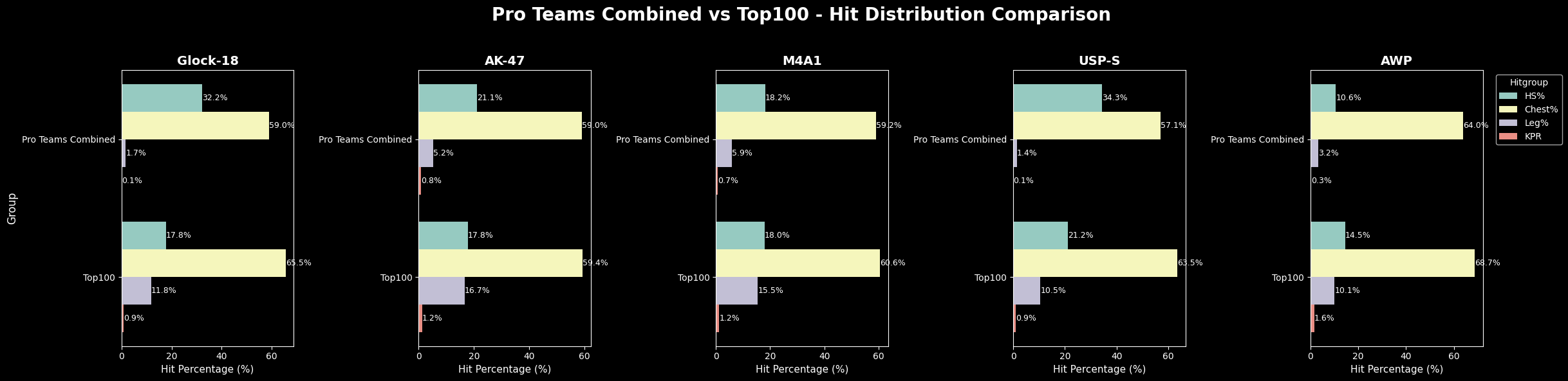
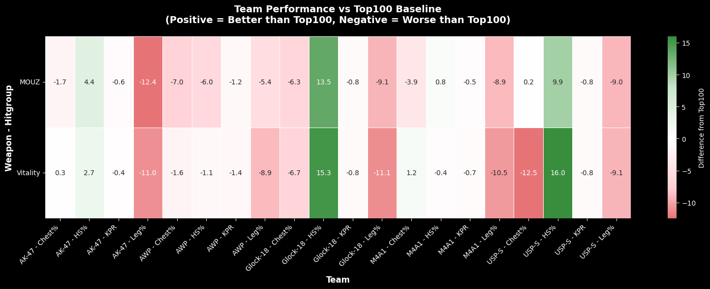
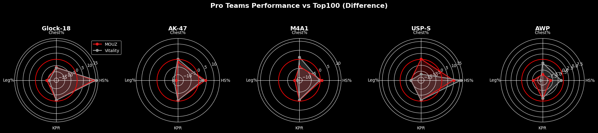
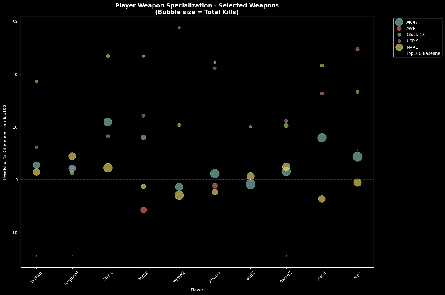
The plot is created for all the pro players combined and Top 100 players. While it may be important to visualize on a per player basis, aggregating all the pros helps us compare pro vs top 100 players better.
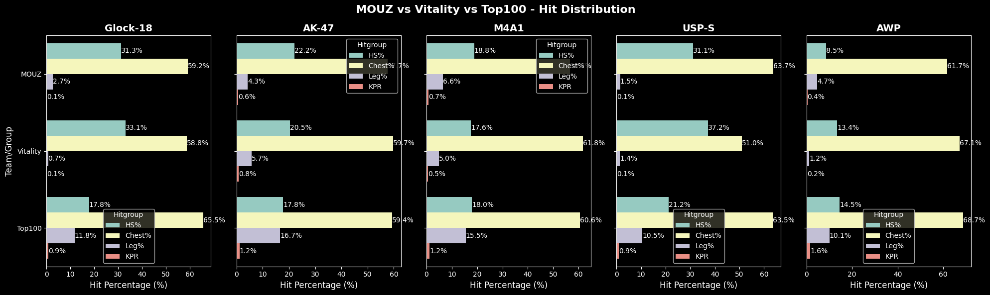
To compare between the winning and the 2nd place team, we also created visualization for that below
fig, axes = plt.subplots(1, 5, figsize=(25, 6))fig.suptitle('Pro Teams Combined vs Top100 - Hit Distribution Comparison', fontsize=20, fontweight='bold', y=0.98)weapons_viz = ["Glock-18","AK-47","M4A1","USP-S","AWP"]for i, weapon inenumerate(weapons_viz): weapon_data = melted_comparison[melted_comparison["Weapon"] == weapon]iflen(weapon_data) ==0: axes[i].text(0.5, 0.5, f'No data for {weapon}', ha='center', va='center', transform=axes[i].transAxes) axes[i].set_title(f'{weapon}', fontsize=14, fontweight='bold')continue sns.barplot(data=weapon_data, x="Hit Percentage", y="Player", hue="Hitgroup", order=["Pro Teams Combined", "Top100"], hue_order=["HS%", "Chest%", "Leg%", 'KPR'], ax=axes[i]) axes[i].set_title(f'{weapon}', fontsize=14, fontweight='bold') axes[i].set_xlabel('Hit Percentage (%)', fontsize=11)if i ==0: axes[i].set_ylabel('Group', fontsize=12)else: axes[i].set_ylabel('')for container in axes[i].containers: axes[i].bar_label(container, fmt='%.1f%%', fontsize=9)if i ==len(weapons_viz) -1: axes[i].legend(title='Hitgroup', bbox_to_anchor=(1.05, 1), loc='upper left')else: axes[i].get_legend().remove()plt.tight_layout(rect=[0, 0, 0.98, 0.95])plt.show()
Import grenades dataset. And drop duplicate entity_id. Entity id provides unique ids for each grenade in a game. So removing duplicate allows us to only have data for 1 grenade per round per map. Although it may be necessary to keep the original dataset, for our analysis, we only needed one datapoint per entity_id.
First, clean up the dataset including changing grenade names into something more redable. The parser parsed the grenade names differently based on the side the thrower was in so we combined each grenade types into one.
vit_util_stats = vit_map_stats.merge(vit_util, how ="left")mouz_util_stats = mouz_map_stats.merge(mouz_util, how ="left")vit_util_stats
map
CT-Win
T-Win
CT-Played
T-Played
T-Win%
CT-Win%
Rounds-Played
Round-Win%
Team
flash
grenade
incendiary
smoke
0
dust2
18
21
36
29
72.4
50.0
65
60.00
vitality
14
11
10
29
1
inferno
27
25
45
40
62.5
60.0
85
61.18
vitality
154
137
172
161
2
mirage
22
16
34
28
57.1
64.7
62
61.29
vitality
15
12
15
20
3
nuke
12
8
19
23
34.8
63.2
42
47.62
vitality
35
25
35
33
4
train
2
4
7
9
44.4
28.6
16
37.50
vitality
13
7
6
26
Add utility damages to the dataframe.
def add_util_damage(df, team_name, drop): damages_df =None assist =None grenades = ['hegrenade', 'smokegrenade', 'inferno', 'molotov','flashbang'] grenade_map = {"hegrenade": "grenade_dmg","smokegrenade": "smoke_dmg","inferno": "incendiary_dmg","molotov": "incendiary_dmg","flashbang":"flash_dmg"}if team_name =="mouz": damages_df = df_damages_mouz.groupby(["map", "weapon"])["dmg_health_real"].sum().reset_index() assist = df_kills_mouz.groupby("map")["assistedflash"].sum().reset_index(name ="assisted_flash_kills")elif team_name =="vitality": damages_df = df_damages_vitality.groupby(["map", "weapon"])["dmg_health_real"].sum().reset_index() assist = df_kills_vitality.groupby("map")["assistedflash"].sum().reset_index(name ="assisted_flash_kills") util_damage = damages_df[damages_df["weapon"].isin(grenades)].copy() util_damage["grenade"] = util_damage["weapon"].map(grenade_map) util_damage = util_damage.groupby(["map", "grenade"])["dmg_health_real"].sum().reset_index()#pivot to match df pivotted_util_damage = util_damage.pivot(index ="map", columns ="grenade", values ="dmg_health_real").reset_index().fillna(0) merged = df.merge(pivotted_util_damage, how ="left") merged = merged.merge(assist, how ="left")#calculate utility damage per round dmg_col = [x for x in merged.columns if"dmg"in x]for x in dmg_col: merged[x] =round(merged[x] / merged["Rounds-Played"],4) merged = merged.drop(drop, axis=1)return merged
At the end, we complined aggregated dataset for rounds and utility datasets. This gives a clean picture of utility usages and their effectiveness in dealing damage.
Couple things to note, in a typical game, decoy is rarely bought since it takes up valuable and limited utility spots and it serves nearly no purpose.
This function does similar to what we calculated earlier. But rather than aggregating the data, we left the rows as is and merged additional round data (utility count and damage) onto it.
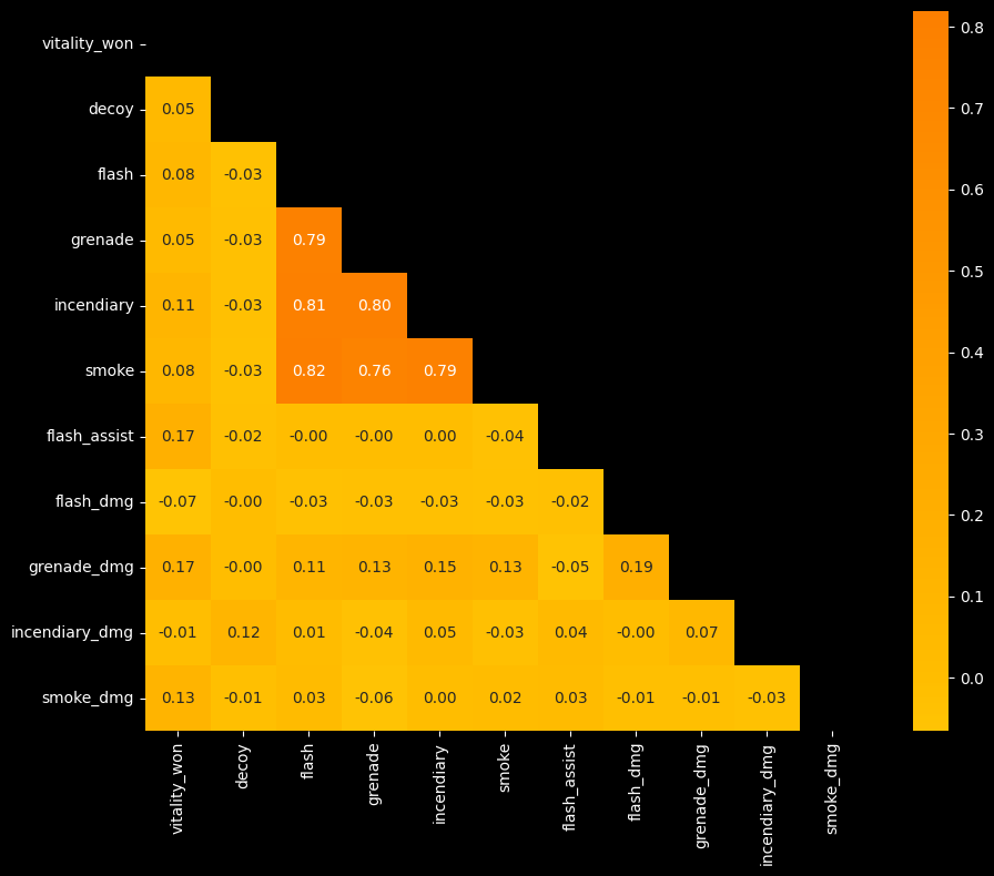
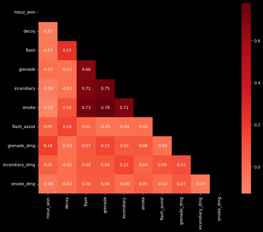
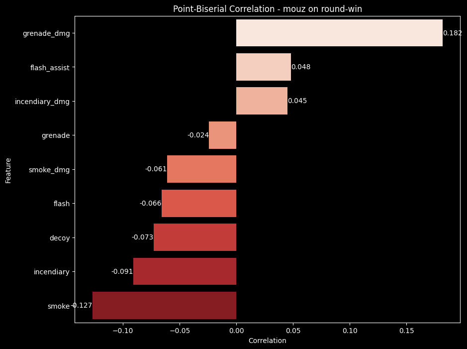
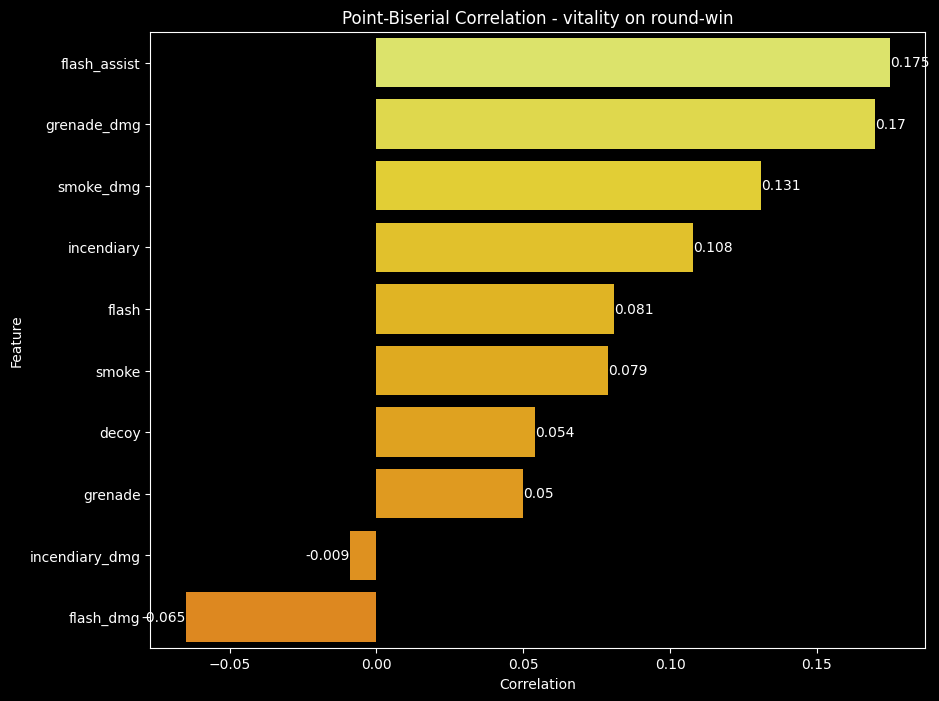
Since the major focus of the project was to see utility’s influce on round outcome, we landed on point biserial, which is good for binary dataset (round win or loss). Also in using barchart rather than a correlation matrix, it is easier to see each utility’s effect on the round outcome.
from scipy.stats import pointbiserialrdef plot_pointbiserial(df, team_name): numeric_cols = df.select_dtypes(include=[np.number]).columns.drop([f"{team_name}_won"]) corr = []for col in numeric_cols: r,p = pointbiserialr(df[f"{team_name}_won"], df[col]) corr.append({"feature": col, "correlation": round(r,3), "p-value": p}) corr_df = pd.DataFrame(corr).sort_values(by="correlation", ascending=False) color ="Reds"if team_name =="mouz"else"Wistia" plt.figure(figsize=(10, 8)) ax = sns.barplot(data = corr_df, x="correlation", y ="feature", palette = color, hue ="feature", legend =False )for container in ax.containers: ax.bar_label(container) plt.title(f"Point-Biserial Correlation - {team_name} on round-win") plt.xlabel("Correlation") plt.ylabel("Feature") plt.show()